Channel Modeling
End-to-End System Overview
Channel Encoding
In digital communication systems, the discrete channel encoder plays a critical role in preparing a binary information sequence for transmission over a noisy channel.
The primary function of the encoder is to introduce redundancy into the binary sequence in a controlled and systematic manner.
This redundancy refers to additional bits that do not carry new information but are strategically added to enable the receiver to detect and correct errors caused by noise and interference during transmission.
Without such redundancy, the receiver would have no means to distinguish between the intended signal and the distortions introduced by the channel, rendering reliable communication impossible in the presence of noise.
The encoding process involves segmenting the input binary information sequence into blocks of bits, where represents the number of information bits per block.
Each unique -bit sequence is then mapped to a corresponding -bit sequence, known as a codeword, where
This mapping ensures that each possible -bit input has a distinct -bit output, preserving the uniqueness of the information while embedding redundancy.
For example, a simple repetition code might map a single bit (e.g., , input ) to a three-bit codeword (e.g., , output ), repeating the bit to add redundancy.
Code Rate
The amount of redundancy introduced by this encoding process is quantified by the ratio .
This ratio indicates how many total bits () are transmitted for each information bit ().
A higher implies more redundancy; for instance, if and , then
meaning 1.75 bits are sent per information bit, with 0.75 bits being redundant.
The reciprocal of this ratio, , is defined as the code rate, denoted :
The code rate measures the efficiency of the encoding scheme, representing the fraction of the transmitted bits that carry actual information.
For the example above (, ),
meaning approximately 57.1% of the transmitted bits are information, and the remaining 42.9% are redundancy.
A code rate closer to 1 indicates less redundancy (higher efficiency), while a lower indicates more redundancy (better error protection but lower efficiency).
The choice of balances the trade-off between data throughput and error resilience, depending on the channel’s noise characteristics.
Modulation and Interface to the Channel
The binary sequence output from the channel encoder, consisting of -bit codewords, is passed to the modulator, which serves as the interface between the digital system and the physical communication channel (e.g., a wireless medium or optical fiber).
The modulator’s role is to convert the discrete binary sequence into a continuous-time waveform suitable for transmission over the channel.
In its simplest form, the modulator employs binary modulation, where each bit in the sequence is mapped to one of two distinct waveforms:
A binary is mapped to waveform .
A binary is mapped to waveform .
For example, in binary phase-shift keying (BPSK), and might be sinusoidal signals differing in phase (e.g., and ), transmitted over a symbol duration .
This one-to-one mapping occurs at a rate determined by the bit rate of the encoded sequence.
Alternatively, the modulator can operate on blocks of bits at a time, using -ary modulation, where represents the number of possible waveforms.
Each unique -bit block is mapped to one of distinct waveforms.
For instance, if , then , and the modulator might use four waveforms (e.g., in quadrature phase-shift keying, QPSK), such as , each corresponding to a 2-bit sequence .
This increases the data rate per symbol—since each waveform carries bits—but requires a more complex receiver to distinguish between the signals.
At the receiving end, the transmitted waveform is corrupted by channel effects (e.g., noise, fading, or interference), resulting in a channel-corrupted waveform.
The demodulator processes this received signal and converts each waveform back into a form that estimates the transmitted data symbol.
In binary modulation, the demodulator might output a scalar value (e.g., a voltage level) indicating whether or was more likely sent.
In -ary modulation, it might produce a vector in a signal space (e.g., coordinates in a constellation diagram) representing one of the possible symbols.
This output serves as an estimate of the original binary or -ary data symbol, though it may still contain errors due to channel noise.
Mathematical Pipeline of the End-to-End Process
Source Input (Information Bits):
The source input is represented as a binary sequence:
This sequence is segmented into blocks, each containing bits.
Channel Encoding.
Each -bit block is encoded into an -bit codeword using a generator matrix:
where is the generator matrix over the binary field.
The resulting output bitstream is:
Bitstream Grouping for Modulation:
The bitstream is grouped into symbols, where each symbol consists of bits:
If , the bitstream is padded with zeros to ensure its length is divisible by .
Symbol Mapping (8-QAM):
Each -bit group is mapped to a complex constellation point using the mapping function μ:
where μ assigns -bit groups to points in an 8-QAM constellation.
Transmission:
The simplified transmitted signal is constructed as:
where denotes the carrier frequency, and represents the real part of the complex expression.
Typically, for passband transmission, , where is a pulse-shaping filter and is the symbol duration.
Example: (7,4) Linear Block Code with 8-QAM Modulation
System Parameters
Channel code:
Code rate:
Modulation: 8-QAM
Modulation order: , bits per symbol:
Using (7,4) Linear Block Code.
A (7,4) linear block code introduces redundancy to facilitate error correction:
: Number of message (information) bits.
: Length of each encoded codeword.
: Number of parity (redundant) bits.
For each 4-bit message, the encoder generates a 7-bit codeword. For example, in systematic encoding:
where are parity bits computed from the message bits using the generator matrix.
Bitstream Formation
The encoder processes a sequence of message bits, dividing it into 4-bit blocks.
Each block is encoded into a 7-bit codeword. For example:
Input messages: 1011, 0010, 1100
Encoded codewords: 1011100, 0010110, 1100101
These codewords are concatenated into a continuous binary stream:
This bitstream is then forwarded to the modulator.
Modulator Input: Preparing for 8-QAM
For 8-QAM:
Each symbol transmits 3 bits (, ).
Symbols correspond to unique points in an 8-point constellation, typically arranged asymmetrically or as a modified rectangular/circular pattern in the I-Q plane.
Mapping Encoded Bits to 8-QAM Symbols
Since the codeword length (7 bits) is not a multiple of 3, the bitstream is treated as continuous and grouped into 3-bit segments:
Grouped into 3-bit segments:
In this example, the total bit count (21 bits) is divisible by 3, so no padding is required. Each 3-bit group is mapped to a unique 8-QAM constellation point, such as:
Each symbol is defined by its amplitude and phase for carrier modulation.
Modulation and Transmission
Each 3-bit group modulates a carrier wave:
The carrier’s amplitude and phase are determined by the corresponding constellation point (e.g., ).
The signal is transmitted over the physical medium (e.g., wireless channel, cable, or optical link).
During transmission, the signal may be subject to noise, fading, or distortion.
Receiver Side (Overview) At the receiver:
Each received analog symbol is demodulated into a 3-bit group.
The demodulated bitstream is re-segmented into 7-bit codewords.
The decoder verifies and corrects errors in each 7-bit codeword using the (7,4) code structure.
The original 4-bit message blocks are recovered.
Additional Steps
Depending on the system, optional preprocessing or enhancements may be applied between encoding and modulation:
Interleaving: Rearranges bits to mitigate burst errors.
Scrambling: Prevents long sequences of 0s or 1s to enhance synchronization.
Framing: Adds synchronization headers or delimiters to assist receiver alignment.
Rate Matching: Adjusts the bit rate to match channel bandwidth (less common in fixed systems like (7,4) + 8-QAM).
Transmission:
Each symbol is transmitted over the channel using its associated I-Q modulation.
Table 1:Summary of The Pipeline
| Stage | Operation |
| Encoder | (7,4) linear block coding |
| Bitstream | Concatenate 7-bit codewords |
| Modulator | Group bits into 3-bit segments |
| Symbol Mapping | Map 3-bit groups to 8-QAM constellation |
| Channel | Transmit analog modulated signal |
| Receiver | Demodulate + decode |
Detection and Decision-Making
The output of the demodulator is fed to the detector, which interprets the estimate and makes a decision regarding the transmitted symbol.
Hard Decision
In the simplest scenario, for binary modulation, the detector determines whether the transmitted bit was a or a based on the scalar output of the demodulator.
For example, if the demodulator provides a value and a threshold τ is established (e.g., in BPSK), the detector decides:
This binary decision is referred to as a hard decision, as it commits definitively to one of two possible outcomes without retaining any ambiguity.
The detection process can be regarded as a form of quantization.
In the hard-decision case, the continuous output of the demodulator (e.g., a real-valued voltage) is quantized into one of two levels, analogous to binary quantization.
The decision boundary (e.g., τ) divides the output space into two regions, each corresponding to a specific bit value.
More generally, the detector can quantize the demodulator output into levels, forming a -ary detector. When -ary modulation is employed (with waveforms), the number of quantization levels must satisfy to distinguish all possible symbols.
For instance, in QPSK (), a hard-decision detector might utilize to map the vector output of the demodulator to one of four symbols.
Soft Decision
In the extreme case, if no quantization is performed (), the detector forwards the unquantized, continuous output directly to the subsequent stage, preserving all information provided by the demodulator.
When , the detector offers greater granularity than the number of transmitted symbols, resulting in a soft decision.
For example, in QPSK (), a detector with might assign the demodulator output to one of eight levels, providing finer resolution within each symbol’s decision region.
Soft decisions retain more information regarding the likelihood of the received signal rather than enforcing a definitive choice, which can enhance error correction in subsequent decoding processes.
The quantized output of the detector—whether hard or soft—is then passed to the channel decoder.
The decoder leverages the redundancy introduced by the encoder (e.g., the additional bits in each -bit codeword) to correct errors induced by channel disturbances.
For hard decisions, the decoder operates with binary or -ary symbols, employing techniques such as Hamming distance minimization.
For soft decisions, it can utilize probabilistic methods, such as maximum likelihood decoding or log-likelihood ratios, to exploit the additional information, typically achieving superior performance in noisy conditions.
Channel Models
A communication channel serves as the medium through which information is transmitted from a sender to a receiver.
The channel’s behavior is mathematically modeled to predict and optimize system performance.
A general communication channel is characterized by three key components:
Set of Possible Inputs : This is the input alphabet, denoted , which comprises all possible symbols that can be transmitted into the channel.
For instance, in a binary system, , indicating that the input is restricted to two symbols. The input alphabet defines the domain of signals that the transmitter can send.
Set of Possible Channel Outputs : This is the output alphabet, denoted , which encompasses all possible symbols that can be received from the channel.
In certain cases, may differ from (e.g., due to noise altering the signal), but in simple models such as binary channels, might also be . The output alphabet represents the range of observable outcomes at the receiver.
Conditional Probability: The relationship between inputs and outputs is captured by the conditional probability
where is an input sequence of length and is the corresponding output sequence of length .
This probability distribution specifies the likelihood of receiving a particular output sequence given a specific input sequence .
It encapsulates the channel’s behavior, including effects such as noise, interference, or distortion, and applies to sequences of any length .
Probabilistic Channel Model.
These components , and the conditional probability provide a complete probabilistic model of the channel, enabling the analysis of how reliably information can be transmitted.
The channel’s characteristics determine the strategies required for encoding, modulation, and decoding to achieve effective communication.
Memoryless Channels
A channel is classified as memoryless if its output at any given time depends solely on the input at that same time, with no influence from previous inputs or outputs.
Mathematically, a channel is memoryless if the conditional probability of the output sequence given the input sequence factors into a product of individual conditional probabilities:
Here, is the probability of receiving output given input at time index , and the product form indicates that each output is statistically independent of all other inputs () and outputs (), conditioned on .
This property implies that the channel has no “memory” of past transmissions; the effect of an input on the output is isolated to that specific time instance.
In other words, for a memoryless channel, the output at time depends solely on the input at time , and the channel’s behavior at each time step is governed by the same conditional probability distribution .
This simplifies analysis and design, as the channel can be characterized by a single-symbol transition probability rather than a complex sequence-dependent model.
The simplest and most widely studied memoryless channel model is the binary symmetric channel (BSC).
In the BSC, both the input and output alphabets are binary, i.e., .
The BSC can be defined with the crossover probability as:
This model is particularly suitable for systems employing binary modulation (where bits are mapped to two waveforms) and hard decisions at the detector (where the receiver makes a definitive choice between 0 and 1).
The BSC captures the essence of a basic digital communication channel with symmetric error characteristics, making it a foundational concept in information theory and coding.
The Binary Symmetric Channel (BSC) Model
The binary symmetric channel (BSC) model emerges when a communication system is considered as a composite channel, incorporating the modulator, the physical waveform channel, and the demodulator/detector as an integrated unit.
This abstraction is particularly relevant for systems with the following components:
Modulator with Binary Waveforms: The modulator maps each binary input 0 or 1 to one of two distinct waveforms (e.g., for 0 and for 1), as in binary phase-shift keying (BPSK).
This converts the discrete binary sequence into a continuous-time signal for transmission.
Detector with Hard Decisions: The receiver’s demodulator processes the channel-corrupted waveform and produces an estimate, which the detector then quantizes into a binary decision (0 or 1), committing to one of the two possible symbols without ambiguity.
In this setup, the physical channel is modeled as an additive noise channel, where the transmitted waveform is perturbed by random noise (e.g., additive white Gaussian noise, AWGN).
The demodulator and detector together transform the noisy waveform back into a binary sequence.
The resulting composite channel operates in discrete time, with a binary input sequence (from the encoder) and a binary output sequence (from the detector).
This end-to-end system abstracts the continuous-time waveform transmission into a discrete-time model, simplifying analysis.
The BSC model assumes that the combined effects of modulation, channel noise, demodulation, and detection can be represented as a single discrete-time channel with binary inputs and binary outputs.
This abstraction is valid when the noise affects each transmitted bit independently, and the detector’s hard decisions align with the binary nature of the input, making the BSC an appropriate and widely utilized model for such systems.
Characteristics of the Binary Symmetric Channel
The composite channel, modeled as a binary symmetric channel (BSC), is fully characterized by the following:
Input Alphabet: , the set of possible binary inputs fed into the channel (e.g., the encoded bits from the transmitter).
Output Alphabet: , the set of possible binary outputs produced by the detector after processing the received signal.
Conditional Probabilities: A set of probabilities that define the likelihood of each output given each input, capturing the channel’s error behavior.
For the BSC, the channel noise and disturbances are assumed to cause statistically independent errors in the transmitted binary sequence, with an average probability of error , known as the crossover probability.
The conditional probabilities are symmetric and defined as:
These probabilities can be interpreted as follows:
: The probability that an input is received as a (an error).
: The probability that an input is received as a (an error).
: The probability that an input is correctly received as a .
: The probability that an input is correctly received as a .
The symmetry arises because the error probability is identical in both directions ( and ), and the correct reception probability is .
Since the channel is memoryless, these probabilities apply independently to each transmitted bit, consistent with:
The BSC is often depicted diagrammatically as a transition model with two inputs and two outputs, connected by arrows labeled with probabilities and .

Channel diagram of the BSC considered above.
The cascade of the binary modulator, waveform channel, and binary demodulator/detector is thus reduced to this equivalent discrete-time channel, the BSC.
This model simplifies the analysis of error rates and informs the design of error-correcting codes, as (typically ) quantifies the channel’s reliability.
Discrete Memoryless Channels (DMC)
The binary symmetric channel (BSC), discussed previously, is a specific instance of a broader class of channel models known as the discrete memoryless channel (DMC).
A DMC is characterized by two key properties:
Discrete Input and Output Alphabets: The input alphabet and output alphabet are finite, discrete sets.
For example, might consist of symbols (e.g., ), and might consist of symbols (e.g., ), where and are integers.
Memoryless Property: The channel’s output at any given time depends only on the input at that same time, with no dependence on prior inputs or outputs.
Mathematically, this is expressed as:
for an input sequence and output sequence .
A practical example of a DMC arises in a communication system using an -ary memoryless modulation scheme.
Here, the modulator maps each input symbol from (with ) to one of distinct waveforms (e.g., in -ary phase-shift keying, M-PSK).
The detector processes the received waveform and produces an output symbol from , consisting of -ary symbols (e.g., after hard or soft quantization, where , ensures all inputs can be distinguished).
The composite channel—comprising the modulator, physical channel, and detector—is thus a DMC, as the modulation and detection processes preserve the discrete and memoryless nature of the system.
The input-output behavior of the DMC is fully described by a set of conditional probabilities , where and .
There are such probabilities, one for each possible input-output pair.
For instance, if (binary input) and (binary output), as in the BSC, there are probabilities (e.g., ).
These conditional probabilities can be organized into a probability transition matrix , where:
The rows correspond to inputs , with .
The columns correspond to outputs , with .
Each entry is the probability of receiving output given input .
The matrix has dimensions (e.g., for the BSC), and each row sums to 1 (i.e., for each ), since these rows represent probability distributions over for a given .
This matrix, often illustrated as in the following figure, provides a compact representation of the DMC’s statistical behavior and facilitates analysis of error rates and channel capacity.
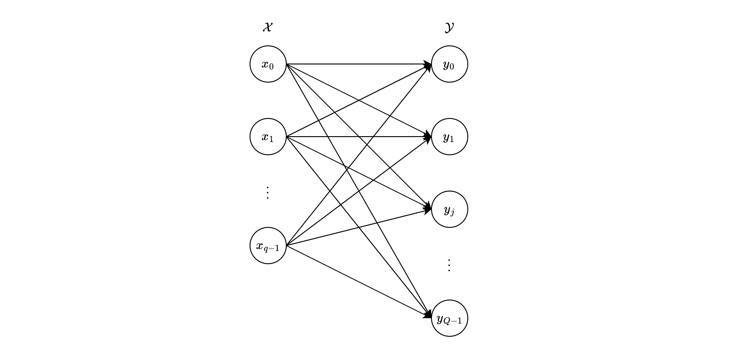
Channel diagram of the considered DMC.
Discrete-Input, Continuous-Output Channels
In contrast to the DMC, the discrete-input, continuous-output channel model relaxes the constraint on the output alphabet while retaining a discrete input.
This model is defined by:
Discrete Input Alphabet: The input to the modulator is selected from a finite, discrete set , with .
For example, in QPSK (), , where each symbol corresponds to a unique waveform.
Continuous Output Alphabet: The detector’s output is unquantized, meaning , the set of all real numbers.
This occurs when the demodulator produces a continuous-valued estimate (e.g., a voltage or likelihood measure) without subsequent quantization into discrete levels.
This configuration defines a composite discrete-time memoryless channel, consisting of the modulator, physical channel, and detector.
The channel takes a discrete input and produces a continuous output .
Its behavior is characterized by a set of conditional probability density functions (PDFs):
For each input symbol , is a PDF over the real line, describing the likelihood of observing a particular output value given .
Unlike the DMC’s discrete probabilities , here is a continuous function, and the probability of falling in an interval is:
with:
This model is relevant when the receiver retains the full resolution of the received signal (e.g., soft-decision outputs) rather than forcing a discrete decision, providing more information for subsequent decoding processes.
Additive White Gaussian Noise (AWGN) Channel
The additive white Gaussian noise (AWGN) channel is one of the most fundamental examples of a discrete-input, continuous-output memoryless channel in communication theory.
Assuming a specific signal mapping, the channel is modeled by:
where:
is the discrete input drawn from an alphabet (for example, a modulated symbol).
is a zero-mean Gaussian random variable with variance . Its probability density function (PDF) is:
representing the additive noise in the channel.
is the continuous output in .
The term white indicates that the noise has a flat power spectral density (i.e., it is uncorrelated across time), while Gaussian refers to its normal distribution.
For a given input , the output is a Gaussian random variable with mean and variance , thus:
Multiple Inputs and Outputs
Consider a sequence of inputs , . The corresponding outputs are:
where each is an independent, identically distributed (i.i.d.) Gaussian noise term,
Because the channel is memoryless, the noise in each output depends only on . Formally,
Substituting the Gaussian PDF yields:
This factorization confirms the channel’s memoryless nature, as the joint PDF of the output sequence is the product of individual PDFs, each depending only on the corresponding input.
Role of AWGN Channels
The AWGN channel is a cornerstone of communication theory, providing an accurate model for systems where thermal noise dominates, such as satellite links and wireless channels.
Its importance extends to analyzing modulation schemes (e.g., BPSK, QPSK) with continuous outputs prior to any quantization, forming the basis for many fundamental results in digital communications.
The Discrete-Time AWGN Channel
A discrete-time (continuous-input, continuous-output) additive white Gaussian noise (AWGN) channel is one in which both the input and output take values in the set of all real numbers:
Unlike channels with discrete alphabets, this model permits continuous-valued inputs and outputs, corresponding to a situation with no quantization at either the transmitter or the receiver.
Input–Output Relationship
At each discrete time instant , an input is transmitted over the channel, producing the received symbol:
where represents additive noise.
The noise samples are independent, identically distributed (i.i.d.) zero-mean Gaussian random variables with variance .
Hence, the PDF of each is:
Given an input , the output is a Gaussian random variable with mean and variance .
Thus, its conditional PDF is:
Power Constraint
A key practical limitation in this channel model is the power constraint on the input, expressed as an expected power limit:
which ensures that the transmitter does not exceed a certain average energy . Note that represents average power (energy per unit time), not total energy.
For a sequence of input symbols:
the time-average power is:
where:
is the squared Euclidean norm of .
As grows large, the law of large numbers implies that, with high probability, the time-average power converges to .
Thus, the constraint:
arises naturally.
In simpler terms:
Geometric Interpretation
Geometrically, the set of all allowable input sequences lies within an -dimensional sphere of radius centered at the origin, since:
This spherical boundary in -dimensional space is crucial for understanding both the channel capacity and the design of signal constellations under energy constraints.
The AWGN Waveform Channel
The AWGN waveform channel describes a physical communication medium in which both the input and output are continuous-time waveforms, rather than discrete symbols.
This can be interpreted as a continuous-time, continuous-input, continuous-output AWGN channel.
To highlight the core behavior of the physical channel, the modulator and demodulator are treated as separate from the channel model, directing attention solely to the process of waveform transmission.
Suppose the channel has a bandwidth , characterized by an ideal frequency response:
and
This indicates that the channel perfectly transmits signals whose frequency components lie in the interval and suppresses those outside this range.
The input waveform is assumed to be band-limited, such that its Fourier transform satisfies:
ensuring conformity with the channel’s bandwidth.
At the channel output, the waveform is given by:
where is a sample function of an additive white Gaussian noise (AWGN) process.
The noise has a power spectral density:
indicating that its power is distributed uniformly across all frequencies.
For a channel of bandwidth , the noise power confined within the interval is:
As will be clarified later, the discrete-time equivalent of this channel provides a simpler perspective through sampling.
Power Constraint and Signal Representation
The input waveform must obey a power constraint:
which restricts the expected instantaneous power of to .
For ergodic processes, where time averages equal ensemble averages (as is the case for stationary processes), this is expressed as:
Interpreted over an interval of length , this stipulates that the average energy per unit time cannot exceed .
Consequently, this condition aligns with that represented via .
To analyze the channel in probabilistic terms, , , and are expanded in terms of a complete set of orthonormal functions .
When a signal has bandwidth and duration , its dimension in signal space can be approximated by .
This approximation follows from the sampling theorem:
A band-limited signal can be reconstructed from samples taken at the Nyquist rate, i.e., samples per second.
Over a time interval , this yields samples, each corresponding to one dimension of the signal space.
Thus, the signal space effectively has dimensions per second.
Orthonormal Expansion
Using this orthonormal set, the waveforms can be written as:
where are orthonormal basis functions (e.g., sinc functions or prolate spheroidal wave functions) satisfying:
The expansion coefficients are:
representing the projections of the signals onto these basis functions.
Since , substituting the expansions into this relationship results in:
By orthonormality, matching coefficients across the sums yields:
Because is white Gaussian noise with power spectral density , the noise coefficients are independent and identically distributed (i.i.d.) Gaussian random variables with zero mean and variance .
Hence, each dimension of the expansion carries a noise variance of , consistent with the total noise power spread over the channel’s bandwidth.
Equivalent Discrete-Time Channel
The AWGN waveform channel can be reduced to a discrete-time model in which each output coefficient is related to the corresponding input coefficient through:
The conditional probability density function (PDF) for each output symbol given the input symbol is:
because:
Since the noise coefficients are independent for different values of , the overall channel is memoryless, which gives:
Vector AWGN Model
From the relationship:
this can be rewritten in a compact vector form:
where:
is the input vector (coefficients from orthonormal expansion),
is the output vector,
is the noise vector,
is the identity matrix,
Noise is i.i.d. Gaussian, so the covariance matrix is diagonal with entries .
Power Constraint and Parseval’s Theorem
The continuous-time power constraint translates directly to the discrete coefficients.
By Parseval’s theorem, for a signal of duration :
In this interval of length , there are coefficients, so the average power per coefficient is:
Hence:
Solving for , one obtains:
Accordingly, a waveform channel of bandwidth and input power behaves like uses per second of a discrete-time AWGN channel whose noise variance is .
This equivalence establishes the connection between the continuous-time channel and its discrete-time counterpart.